
TL;DR
- Geo-Experiments assign geographic markets randomly to treatment and control conditions, measuring campaign incrementality where user-level holdouts are operationally or technically impossible.
- They are the preferred measurement methodology for TV, radio, OOH, and broad digital campaigns — channels where individual user exclusion distorts auction dynamics or lacks platform support.
- Executed correctly, geo-experiments reduce blended CAC by 15–30% by exposing zero-lift channel spend that attribution models consistently misattribute as high-performing.
What Is Geo-Experiments?
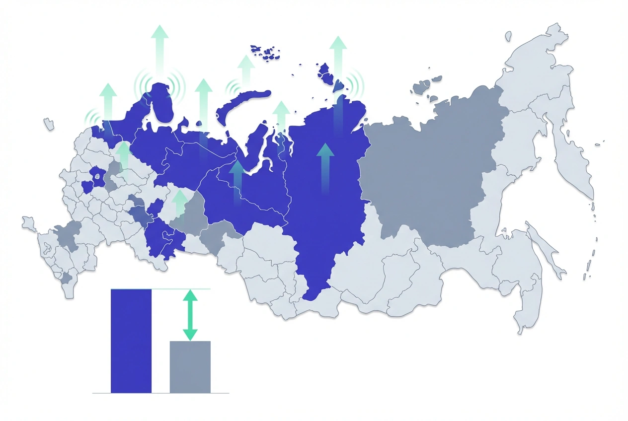
Geo-Experiments are a causal inference methodology in which geographic units — cities, DMAs, states, or countries — are randomly assigned to either a treatment condition (campaign active) or a control condition (campaign withheld), enabling a clean comparison of lead generation outcomes between the two groups.
The fundamental logic mirrors a randomized controlled trial (RCT), but the unit of randomization shifts from the individual user to the geographic market. This makes geo-experiments the only viable incrementality measurement approach for channels that cannot support user-level holdouts.
Where user-level holdout testing requires platform infrastructure and individual tracking continuity, geo-experiments require only geographic campaign targeting controls — making them applicable across virtually every marketing channel including offline.
Test LeadSources today. Enter your email below and receive a lead source report showing all the lead source data we track—exactly what you’d see for every lead tracked in your LeadSources account.
How Geo-Experiments Work
The design process begins with market selection and matching — the most technically demanding phase of any geo-experiment.
Before the campaign launches, available geographic markets are analyzed for pre-experiment similarity across key metrics:
- Historical lead volume and CVR trends
- Baseline MQL and pipeline generation rates
- Seasonal conversion patterns
- Demographic and firmographic audience composition
- Competitive advertising density by market
Matched market pairs — or larger balanced groups — are then randomly assigned to treatment or control conditions. The campaign runs in treatment markets while control markets receive no exposure.
At study close, the incremental impact is calculated using a Difference-in-Differences (DiD) framework:
Treatment Effect = (Post_treatment − Pre_treatment) − (Post_control − Pre_control)This approach isolates campaign-driven lift by controlling for both pre-existing market differences and external time trends that affect all markets equally.
Worked example: A B2B SaaS company tests a regional TV campaign across six matched DMA pairs.
- Treatment DMAs: lead CVR moves from 2.1% (pre) to 2.9% (post) → +0.8 pp
- Control DMAs: lead CVR moves from 2.0% (pre) to 2.2% (post) → +0.2 pp
- DiD estimate: 0.8 − 0.2 = +0.6 pp incremental lift
- Relative Lift: 0.6 / 2.0 = 30% incremental CVR improvement
Why It Matters for Lead Attribution
Attribution models fail categorically for offline and broadcast channels. There is no pixel, no click, no trackable touchpoint connecting a TV impression to a CRM lead record.
Yet TV, radio, OOH, and podcast advertising collectively represent a significant share of enterprise B2B marketing budgets. Without geo-experiments, spend in these channels is either blindly maintained, cut on gut instinct, or misattributed to digital touchpoints that happened to follow offline exposure.
Geo-experiments solve the attribution gap directly. By comparing lead generation rates across geographically separated treatment and control markets, they produce a market-level counterfactual — the conversion rate in a world where the campaign never ran — that no touchpoint model can replicate.
The business impact is material. Analytic Partners’ cross-industry analysis shows that marketers who measure offline channels through geo-based methods routinely discover that 20–40% of offline spend produces zero measurable incremental lift. Redirecting that budget to validated high-lift channels typically reduces blended CAC by 15–25% within a single planning cycle.
Geo-experiments are equally valuable for digital channels in privacy-constrained environments. As third-party cookie deprecation limits user-level tracking, geo-based measurement provides a scalable, privacy-compliant alternative for validating digital channel incrementality at scale.
Design Variants and Architectures
Three primary design approaches exist, each optimized for a different measurement context.
| Design Type | Structure | Best Application | Key Limitation |
|---|---|---|---|
| Matched Market Pairs | Markets paired by similarity; one assigned treatment, one control | TV, OOH, radio — 2–8 market pairs | Low statistical power with few pairs; sensitive to market shocks |
| Randomized Geo Split | Large pool of markets randomly split into treatment and control groups | Digital geo-targeting, national B2B campaigns | Requires sufficient market count (typically 20+) for valid randomization |
| Synthetic Control | Control group constructed algorithmically from weighted combination of non-treated markets | Single-market interventions; sparse geography programs | Model-dependent; requires extensive pre-experiment time series data |
For most B2B programs with regional market structures, matched market pairs offer the best balance of operational simplicity and measurement validity, provided markets are rigorously matched on pre-experiment lead metrics.
Statistical Design and Sample Size
The statistical challenge in geo-experiments is fundamentally different from user-level holdout tests. The unit of observation is a market, not a user — and typical B2B programs have access to far fewer markets than users.
With fewer experimental units, achieving adequate statistical power requires either:
- Longer study windows — more pre-experiment data improves matching quality; more post-experiment data accumulates sufficient conversions per market
- Larger market effects — high-spend, high-reach campaigns in large DMAs generate sufficient conversion volume to detect moderate effects
- Covariate adjustment — incorporating pre-experiment lead data as covariates in the analysis reduces residual variance and improves power without requiring additional markets
Google’s GeoX and Meta’s GeoLift open-source libraries provide Bayesian power analysis frameworks specifically designed for geo-experiment sample size estimation.
Minimum viable geo-experiment design for B2B lead programs:
| Parameter | Recommendation |
|---|---|
| Minimum market pairs | 4–6 matched pairs (8–12 total markets) |
| Pre-experiment baseline window | 8–12 weeks of lead data for matching |
| Experiment duration | 4–8 weeks minimum (longer for B2B with 30–90 day sales cycles) |
| Target confidence level | 90% for exploratory tests; 95% for budget reallocation decisions |
| Minimum detectable effect | 15–25% relative lift (geo designs have lower power than user-level tests) |
Implementation: 5-Step Framework
- Define the measurement objective and primary KPI — specify whether you are measuring form submission CVR, MQL volume, pipeline value, or CAC at the market level. The KPI must be trackable at the geographic grain before the experiment launches.
- Select and match markets — identify candidate markets with sufficient lead volume. Use at least 8 weeks of pre-experiment lead data to match markets on CVR, lead volume, and conversion trends. Markets with structurally different audience compositions (e.g., tech-heavy metro vs. manufacturing region) should never be paired.
- Randomize assignment and document the protocol — randomly assign matched pairs to treatment or control conditions. Document the assignment protocol, planned analysis method, and expected treatment effect before any campaign activity begins. Post-hoc design changes invalidate causal interpretation.
- Execute with geographic precision — configure campaign geo-targeting to include only treatment markets. Verify targeting settings weekly during the experiment. Geographic targeting errors that expose control markets are the most common source of validity failure in geo-experiments.
- Analyze using Difference-in-Differences or Bayesian causal inference — apply the DiD estimator to isolate the campaign effect from concurrent market trends. For synthetic control designs, use GeoX or CausalImpact (Google) to model the counterfactual. Report results with confidence intervals, not just point estimates — the uncertainty range is as important as the central estimate for budget decisions.
Common Challenges and Solutions
Geo-experiments introduce validity threats that user-level holdouts do not face. Three challenges dominate.
- Geographic spillover (contamination) — campaign exposure in treatment markets leaks into adjacent control markets through shared media, physical presence, or digital spillover (e.g., cross-market LinkedIn targeting). Mitigation: select control markets with geographic distance or natural barriers (state lines, major metros) from treatment markets.
- Market heterogeneity — imperfect market matching means treatment and control markets differ in ways unrelated to the campaign. Mitigation: use covariate adjustment in the DiD model to control for pre-experiment differences; include market-level fixed effects in the regression.
- External shocks — local events, competitive promotions, or economic disruptions in specific markets during the experiment period confound results. Mitigation: monitor market-level news and competitive activity throughout the experiment; exclude markets that experience identifiable exogenous shocks from the final analysis.
- Small N statistical fragility — with only 4–8 market pairs, a single outlier market can dominate the aggregate result. Mitigation: run sensitivity analyses removing individual markets one at a time (jackknife analysis) to verify result stability.
Geo-Experiments Best Practices
Programs that generate durable, decision-grade geo-experiment results follow a consistent set of design and governance principles.
- Pre-register the full experiment design — market assignment, analysis methodology, primary KPI, expected effect size, and confidence threshold must be documented before any campaign activity begins. Post-hoc analytical changes undermine causal credibility.
- Use CRM lead source tagging at the market level — append geographic market assignment (treatment vs. control) to every lead record at the point of form submission. This enables downstream pipeline and LTV comparison by market cohort, not just top-of-funnel CVR.
- Run sequential experiments to improve power — if the first geo-experiment is underpowered (common with 2–4 market pairs), treat it as a pilot to refine market matching, then run a confirmatory experiment with refined design before making budget commitments.
- Combine with MMM for channel portfolio decisions — geo-experiments validate individual channel incrementality; Marketing Mix Modeling optimizes the cross-channel budget mix. Geo-experiment outputs serve as ground-truth calibration data for MMM model inputs.
- Account for B2B sales cycle lag — in markets where the average MQL-to-SQL cycle is 30–90 days, measuring only form submissions understates downstream pipeline impact. Extend the post-experiment measurement window by at least one full sales cycle to capture the complete revenue effect.
Frequently Asked Questions
How does this approach differ from geo-targeted A/B testing?
Geo-targeted A/B testing compares two versions of a campaign asset — different creatives, offers, or messages — across geographic markets to optimize execution. Geo-experiments compare markets receiving a campaign against markets receiving nothing to determine whether running the campaign at all drives incremental conversions. A/B testing optimizes how a campaign communicates; geo-experiments determine whether the campaign generates measurable ROI.
How many markets are needed for statistical validity?
For matched market pair designs, a minimum of 4–6 pairs (8–12 total markets) provides enough experimental units to achieve reasonable statistical power for moderate effects (15–25% relative lift). Programs with access to 20+ markets can use randomized geo splits, which provide stronger randomization guarantees. Google’s GeoX tool and Meta’s GeoLift library both offer built-in power analysis to determine the minimum market count for a given effect size and confidence level.
Can this method measure B2B lead quality, not just volume?
Yes — but only if CRM data is structured to support market-level cohort comparison. By appending treatment or control market tags to every lead record at form submission and tracking those cohorts through MQL, SQL, and closed-won stages, geo-experiments can compare MQL-to-SQL rates, average deal size, and LTV across market conditions. Programs that measure only top-of-funnel CVR miss the most commercially relevant signal: whether the channel drives revenue, not just form submissions.
How do you handle geographic spillover and market contamination?
Spillover — campaign exposure leaking from treatment to control markets — compresses measured lift toward zero by inflating the control market’s baseline. Prevention strategies include selecting control markets with physical or demographic separation from treatment markets, using DMA-level boundaries that reduce cross-market audience overlap, and monitoring control market lead rates during the experiment for unexplained increases. Post-experiment, cross-reference digital impression data with control market users to quantify contamination levels.
When is this approach preferable to user-level holdout tests?
Geo-experiments are the correct choice when user-level holdouts are technically infeasible (TV, radio, OOH), when platform infrastructure does not support ghost ad architecture, or when privacy regulations restrict individual user tracking. They are also preferable for large-scale brand campaigns where withholding 10–20% of users from a national campaign would meaningfully reduce reach and frequency. For digital channels with platform-native holdout support, user-level holdouts offer higher statistical precision; for everything else, geo-experiments are the operationally viable alternative.
How long should a geographic market experiment run?
Minimum duration is 4 weeks for B2C programs with short conversion cycles. For B2B lead generation — where MQL-to-SQL cycles average 30–90 days — the experiment window should cover at minimum 6–8 weeks of active measurement, followed by a post-experiment tracking window of one full sales cycle to capture downstream pipeline. Ending geo-experiments before pipeline metrics mature systematically understates channel impact and leads to premature spend cuts in channels with long revenue lag.
What tools are available to analyze geo-experiment data?
Google’s GeoX (open source, R package) and Meta’s GeoLift library provide end-to-end geo-experiment analysis including market matching, power analysis, and Bayesian causal inference. Google’s CausalImpact package is widely used for synthetic control estimation in single-market intervention studies. For enterprise programs, third-party measurement vendors including Analytic Partners and Nielsen offer managed geo-experiment services with integrated MMM calibration and reporting.